Tracing the Geometric Algebra Ways
Description: This is a blog that explores the world of geometric algebra using ray tracing

Author: Joran Vandenbroucke
Published on: 2022-11-21
Read Time (Minutes): 10
Tags: Applied Geometric Algebra, Geometric Algebra, GA, Ray Tracing
Applied Geometric Algebra
Chapter 1: Ray Tracing
Welcome to this series of blog posts where we explore random topics and combine two topics that are usually not combined. In this chapter, we will dive into the world of Geometric Algebra and CPU Ray Tracing. For this ray tracer, we will mainly focus on the closest hit and shadow ray, and also have a look at bounding volume hierarchies using geometric algebra. Therefore, a background in ray tracing is recommended. We will use C++ as the implementation language and build upon GLM (OpenGL Math) to make geometric algebra happen. The math expansion that gets created in this chapter is small and easy to use. However, GLM and our expansion can be replaced by the Klein Library for better performance and more accurate results.
Prerequisites
This chapter about Geometric Algebra and Ray Tracing works best if you have a background in programming, math and ray tracing.
Chapter Outline
This chapter consists of seven parts:
- Ray Plane Intersection
- Ray Triangle Intersection
- Shadow Ray
- Camera & movement
- Bounding Volume Hierarchy
- Advanced: Ray Sphere
- Advanced: Multy Geometric Algebra optimizations
The full source code of each final project is available here.
Part 1. Ray Plane Intersection
Geometric Algebra
If you've ever worked with vectors and matrices in math or computer programming, you might be interested to know that there's a newer approach called Geometric Algebra.
In Geometric Algebra, instead of just working with vectors and matrices, you also have a concept called a k-vector, which can represent not just a magnitude and direction like a traditional vector, but also higher-dimensional objects such as planes and volumes.
To help you understand the differences between traditional vector math and Geometric Algebra, let's take a look at the table below:
| Traditional | Geometric Algebra |
|---|---|
| Vector | Vector |
| Matrix | Matrix |
| $A\cdot B+A\times B$ | $A\cdot B+A\wedge B$ |
| x-axis | $\mathbf{e}_{1}$ |
| y-axis | $\mathbf{e}_{2}$ |
| z-axis | $\mathbf{e}_{3}$ |
| w-axis | $\mathbf{e}_{4}$ |
| yz-plane | $\mathbf{e}_{23}$ |
| zx-plane | $\mathbf{e}_{31}$ |
| xy-plane | $\mathbf{e}_{12}$ |
As you can see, many of the concepts from traditional vector math, such as vectors and matrices, are also present in Geometric Algebra.
The first difference is the vector product or the geometric product, but in fact they are the same ... sort of.
In vector algebra and in geometric algebra the dot product is the same $A \cdot B = \lVert A \rVert \lVert B \rVert \cos \theta$, the cross product is actually also the same and $$\begin{equation} \lVert A \times B \rVert = \lVert A \rVert \lVert B \rVert \sin \theta \end{equation}$$ while the wedge product looks like $$\begin{equation}\lVert A \wedge B \rVert = \lVert A \rVert \lVert B \rVert \sin \theta\end{equation}$$
The different between the cross product ($\times$) and wedge product ($\wedge$) is that the wedge is designed to work with any combination of vectors and multivectors.
What is a multi-vector I hear you say. Well a multi-vector is something you get when two or more vectors are combined using the wedge product ($\wedge$).
If you wedge two vectors, you get a 2-vector, also known as a bi-vector and if you wedge three vectors than you get a 3-vector, a 2-vector can also be wedged with a vector or a 2-vector or a 3-vector, and we can go on and on.
Now, the second difference, and this is the difference which makes everything possible, is how we call our axis. instead of using $x$, $y$, $z$ and $w$ we use $\mathbf{e}_{1}$, $\mathbf{e}_{2}$, $\mathbf{e}_{3}$ and $\mathbf{e}_{4}$.
This difference allows us to go beyond four axis without having to think of new axis names, but a bigger difference lies in how we represent the axis.
While $x$, $y$, $z$ and $w$ can be seen as ways to index from a vector as in myVector.x is simular to myVector[x], using $\mathbf{e}_{1}$, $\mathbf{e}_{2}$, $\mathbf{e}_{3}$ and $\mathbf{e}_{4}$ is more like masking things out, like a bitwise mask or a Photoshop mask, this looks the something like myVector*e1.
Let's generalize Geometric Algebra axis as $\mathbf{e}_{i}$, $\mathbf{e}_{i}$ is a vector, how it looks like doesn't matter for us, we will use it like a symbol, just like how $x$, $y$, $z$ and $w$ are also just symbols.
$\mathbf{e}_{i}$ has a cool property and that is that it squares to either $1$, $-1$ or $0$, so $\mathbf{e}_{i}^{2} \in [-1,0,1]$. But how do we know what axis squares to what? To answer that question I would refer you to the Ganja.js cheat-sheets
This cheat-sheet shows us per subalgebra a $\R$ followed by three numbers, they tell us how many axis square to one, negative one and zero respectively.
For our case we are interested in 3D Projective Geometric Algebra and the sheet tels us this is $\R_{3,0,1}$, this mean we have $\mathbf{e}_{1}$, $\mathbf{e}_{2}$ and $\mathbf{e}_{3}$ that squares to one, and we have $\mathbf{e}_{4}$ which squares to zero, because $\mathbf{e}_{4}$ is the only one that squares to zero we will call this $\mathbf{e}_{0}$.
Ray Tracing
After all this math, it's time to actualy start to work on our ray tracer, for this part within the chapter, we need a plan, a line and a point.
A plane looks like $$\begin{equation}a\mathbf{e}_{1} + b\mathbf{e}_{2} + c\mathbf{e}_{3} + d\mathbf{e}_{0}\end{equation}$$with other words, this is your basic glm::vec4 where that x, y and z or a, b and c are the direction of the plane, while w or d is the distance from origine to the plane.
using plane = glm::vec4;
...
now we just need some functions to safely initialize this
...
inline plane make_plane( float x, float y, float z = 0.0f, float w = 0.0f )
{
 return { x, y, z, w };
}
inline plane make_plane( const glm::vec2& v, float z = 0.0f, float w = 0.0f )
{
 return { v, z, w };
}
inline plane make_plane( const glm::vec3& v, float w = 0.0f )
{
 return { v, w };
}
inline plane make_plane( const glm::vec2& v1, const glm::vec2& v2 )
{
 return { v1, v2 };
}
We have everything for a plane now, so lets go to a line.
The line that we will be using exists out of two glm::vec4's, the first one will be the "Euclidean" part of our line, we can use this as our position.
The second part is called the "Ideal" part of the line, this part of a line can be used as directions.
Both the Euclidean and Ideal part have some interesting properties, but I will talk about that in part x.
Before making our line in code, let's look at its definition $$\begin{equation}a\mathbf{e}_{01} + b\mathbf{e}_{02} + c\mathbf{e}_{03} +d\mathbf{e}_{23} + e\mathbf{e}_{31} + f\mathbf{e}_{12}\end{equation}$$
struct line
{
 glm::vec4 euclidean;
 glm::vec4 ideal;
 line( float a, float b, float c, float d, float e, float f ) noexcept
 : euclidean{ c, b, a, 0.0f }
 , ideal{ f, e, d, 0.0f }
 {
 }
};
With the line done, lets create our last object, the point. The point has the following formula $$\begin{equation}x\mathbf{e}_{032} + y\mathbf{e}_{013} + z\mathbf{e}_{021} + \mathbf{e}_{123}\end{equation}$$
This means that we can use a singular glm::vec4 again to create a point.
using point = glm::vec4;
...
One important thing to mention is that, unlike the plane, when creating a point manually, we want w to be one. This is because we are working with homogenous coordinates.
Therefor our make_point functions will look a bit different from the make_plane functions.
...
inline point make_point( float x, float y, float z = 0.0f, float w = 1.0f )
{
 return { x, y, z, w };
}
inline point make_point( const glm::vec2& v, float z = 0.0f, float w = 1.0f )
{
 return { v, z, w };
}
inline point make_point( const glm::vec3& v, float w = 1.0f )
{
 return { v, w };
}
inline point make_point( const glm::vec2& v1, const glm::vec2& v2 )
{
 return { v1, v2 };
}
Voila, most of the work is done, we just need our intersection algorithm, and we are done.
Intersection
So, the intersection algorithm, it's complicated right? No! Not at all!
Because we are using basic/standard formulas for planes, lines and points, we can use the wedge product ($\wedge$).
The wedge product has as side effect that it can calculate the intersection of primitive objects like planes, lines and points.
So in order to find the intersection between a plane and a line we calculate the wedge of a plane and a line, $point = plane \wedge line$
Using a plane $a$ and a line $b$ defined as $$\begin{align}&a=a_1 \mathbf{e}_{1} + a_2 \mathbf{e}_{2} + a_3 \mathbf{e}_{3} + a_4 \mathbf{e}_{0} \\
&b=b_1\mathbf{e}_{01} + b_2\mathbf{e}_{02} + b_3\mathbf{e}_{03} +b_4\mathbf{e}_{23} + b_5\mathbf{e}_{31} + b_6\mathbf{e}_{12}\end{align}$$
We can now write our the outer product as
$$\begin{equation}
a\wedge b=(a_1 \mathbf{e}_{1} + a_2 \mathbf{e}_{2} + a_3 \mathbf{e}_{3} + a_4 \mathbf{e}_{0})\wedge(b_1\mathbf{e}_{01} + b_2\mathbf{e}_{02} + b_3\mathbf{e}_{03} +b_4\mathbf{e}_{23} + b_5\mathbf{e}_{31} + b_6\mathbf{e}_{12})
\end{equation}$$
now it's just a matter of working out the brackets.
$$\begin{equation}
\begin{split}
a\wedge b =
&(a_1 b_1)\mathbf{e}_{1}\wedge\mathbf{e}_{01}+(a_1 b_2)\mathbf{e}_{1}\wedge\mathbf{e}_{02}+(a_1 b_3)\mathbf{e}_{1}\wedge\mathbf{e}_{03} + \\
&(a_1 b_4)\mathbf{e}_{1}\wedge\mathbf{e}_{23}+(a_1 b_5)\mathbf{e}_{1}\wedge\mathbf{e}_{31}+(a_1 b_6)\mathbf{e}_{1}\wedge\mathbf{e}_{12} + \\
&(a_2 b_1)\mathbf{e}_{2}\wedge\mathbf{e}_{01}+(a_2 b_2)\mathbf{e}_{2}\wedge\mathbf{e}_{02}+(a_2 b_3)\mathbf{e}_{2}\wedge\mathbf{e}_{03} + \\
&(a_2 b_4)\mathbf{e}_{2}\wedge\mathbf{e}_{23}+(a_2 b_5)\mathbf{e}_{2}\wedge\mathbf{e}_{31}+(a_2 b_6)\mathbf{e}_{2}\wedge\mathbf{e}_{12} + \\
&(a_3 b_1)\mathbf{e}_{3}\wedge\mathbf{e}_{01}+(a_3 b_2)\mathbf{e}_{3}\wedge\mathbf{e}_{02}+(a_3 b_3)\mathbf{e}_{3}\wedge\mathbf{e}_{03} + \\
&(a_3 b_4)\mathbf{e}_{3}\wedge\mathbf{e}_{23}+(a_3 b_5)\mathbf{e}_{3}\wedge\mathbf{e}_{31}+(a_3 b_6)\mathbf{e}_{3}\wedge\mathbf{e}_{12} + \\
&(a_4 b_1)\mathbf{e}_{4}\wedge\mathbf{e}_{01}+(a_4 b_2)\mathbf{e}_{4}\wedge\mathbf{e}_{04}+(a_4 b_3)\mathbf{e}_{4}\wedge\mathbf{e}_{03} + \\
&(a_4 b_4)\mathbf{e}_{4}\wedge\mathbf{e}_{23}+(a_4 b_5)\mathbf{e}_{4}\wedge\mathbf{e}_{31}+(a_4 b_6)\mathbf{e}_{4}\wedge\mathbf{e}_{12}
\end{split}
\end{equation}$$
With keeping formula (2) in mind, we can clean things up because
$$\begin{equation}
\mathbf{e}_{i}\wedge\mathbf{e}_{i}=0
\hskip 5em
\mathbf{e}_{i}\wedge\mathbf{e}_{j}=-\mathbf{e}_{j}\wedge\mathbf{e}_{i}
\end{equation}
$$
When applying these rules we get that
$$\begin{equation}
\begin{split}
a\wedge b=
&(a_2 b_3 - a_3 b_2 - a_4 b_6)\mathbf{e}_{032}+\\
&(-a_1 b_3 + a_3 b_1 - a_4 b_5)\mathbf{e}_{013}+\\
&(a_1 b_2 - a_2 b_1 - a_4 b_4)\mathbf{e}_{021}+\\
&(a_1 b_6 + a_2 b_5 + a_3 b_4)\mathbf{e}_{123}\\
\end{split}
\end{equation}$$
If we look back at the point than we see that (5) gives us the same outcome as (11).
Great! Now we only deed the distance. Lucky us, we are using projective geometric algebra, which uses homogenous coordinates. This means tha we just need to divide the z by the w
putting this in code we get
inline point operator^( plane a, line b )
{
	return make_point(
		a.y * b.euclidean.z - a.z * b.euclidean.y - a.w * b.ideal.z,
		-a.x * b.euclidean.z + a.z * b.euclidean.x - a.w * b.ideal.y,
		a.x * b.euclidean.y - a.y * b.euclidean.x - a.w * b.ideal.x,
		a.x * b.ideal.z + a.y * b.ideal.y + a.z * b.ideal.x
	);
}
...
float get_distance(const point& point)
{
	return point.z / point.w;
}
I used the ^ operator because it looks like the wedge symbol ($\wedge$) and it is also used in the Klein Library for the wedge product.
Putting this all together we get
// generate planes and colors
plane[6] planes{
    make_plane( 0, 1, 0, -5 ),
    make_plane( 0, -1, 0, -5 ),
    make_plane( 1, 0, 0, -5 ),
    make_plane( -1, 0, 0, -5 ),
    make_plane( 0, 0, 1, -10 ),
    make_plane( 0, 0, -1, -5 )
};
Color[6] colors{ Color{ 1, 0, 0 }, Color{ 0, 1, 1 }, Color{ 0, 1, 0 }, Color{ 1, 0, 1 }, Color{ 0, 0, 1 }, Color{ 1, 1, 0 } };
...
// get ndc coords
...
line  ray{ 0, 0, 0, ndcX, ndcY, -1 };
Color finalColor{};
float closest{ 1e6f };
for ( uint8_t i{}; i < 6; ++i )
{
    point intersection = planes[i]^ray;
    float distance{ intersection.z / intersection.w };
    if ( distance < closest && distance > 0 )
    {
        finalColor = cols[i];
        closest    = distance;
    }
}
// save to image/screen
...
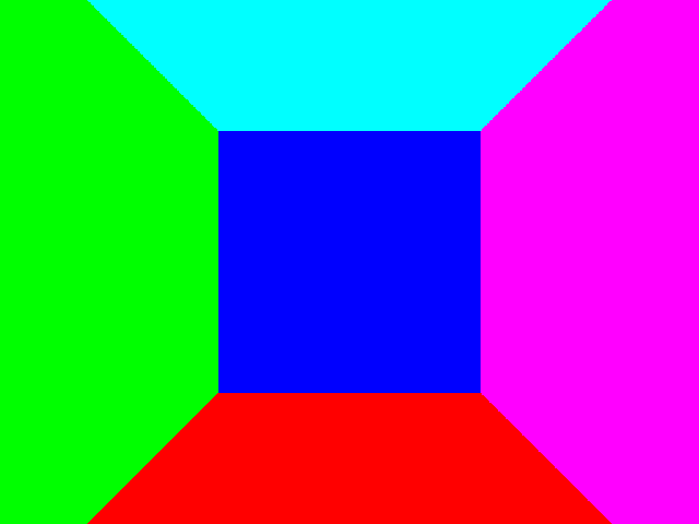
Now that we can draw some planes, let us switch things over to triangles.