Local Clearance Minimum in Recast
Description: This series of blog posts is about Navmeshes. This blog looks at how we can implement it into Recast.

Author: Joran Vandenbroucke
Published on: 2024-07-16
Read Time (Minutes): 10
Tags: LCM, Local Clearance Minimum, Navmesh, Navigation Mesh, Navmesh Generation, Pathfinding, Recast, Detour, Recast & Detour
Navigation Meshes
Part 2: LCM in Recast
Welcome back, adventurer!
In the last post, we explored navmesh generators and learned about the Local Clearance Minimum (LCM). It identifies the narrowest parts of a region, helping us merge navigation meshes for different agents.
As we embark on the second part of our journey, we delve into Recast. Recast is a popular open-source library that has been integrated into Unreal Engine, and now, it is time for us to explore its depths. Our mission? To integrate LCMs into the pipeline using Recast. We will run tests, analyse results, and uncover the strengths and weaknesses of our new algorithm. In Part 3, We will create a new Navmesh generation method using the medial axis to detect LCMs. The medial axis represents a shape's skeleton and is used to identify the tightest spots in the environment where LCMs are needed. This approach can be a modern, dependable, and fast alternative to frameworks like Recast.
Our journey ends in Navigation City. In Part 4, we will use the generated LCMs for pathfinding, taking LCMs into account, which will be different from standard methods.
Navigating the Blogs
Here is what you can expect in each Part:
-
What is the Local Clearance Minimum? - A deep dive into the concept that can change the game.
-
LCM in Recast - Implementing LCMs within the Recast framework.
-
LCM: A Custom Solution from the Ground Up (Work in progress) - Building a Navmesh generator around the LCM concept.
-
Navigating Using the LCM (Work in progress) - The practical implications of pathfinding using LCMs.
Part 2, Chapter 1: How does Recast work?
Our focus in this chapter is the Single Mesh Generator, one of the generator examples of Recast. The Single Mesh Generator has seven steps:
-
Parameter Initialisation: Recast sets the stage, initialising all parameters and variables. These include cell size, height, walkable slope angle, agent height, and radius.
-
Triangle Clean-up & Voxelization: Recast cleans up by removing all triangles with a steep slope. The remaining triangles are transformed into voxels.
-
Mark As Walkable: Recast calculates the walkable surfaces using the voxel data. Some filters are applied to remove floor voxels that are too close to ceiling voxels.
-
Region Partitioning: The walkable space is divided into regions using watershed, monotone, or layer partitioning. Our focus is on the watershed partitioning.
-
Region Tracing to Contour: Each region's contour is traced and simplified. Recast creates an outline that follows the voxel regions and then smooths the edges to remove stair-stepping.
-
Navmesh Generation: Recast creates a polygon mesh from the simplified contour data by triangulating the vertices and removing duplicates.
-
Detailed Navmesh Generation: The poly mesh and height field are combined to make a more detailed mesh with accurate height data.
Once the navmesh is generated, it is handed over to Detour, the integrated pathfinding library. Detour then uses this detailed navmesh for efficient game or application pathfinding.
Part 2, Chapter 2: LCM Extraction Method
In our previous adventure, we learned that we needed the medial axis to extract the LCMs. We saw that the medial axes looked similar to the distance map.
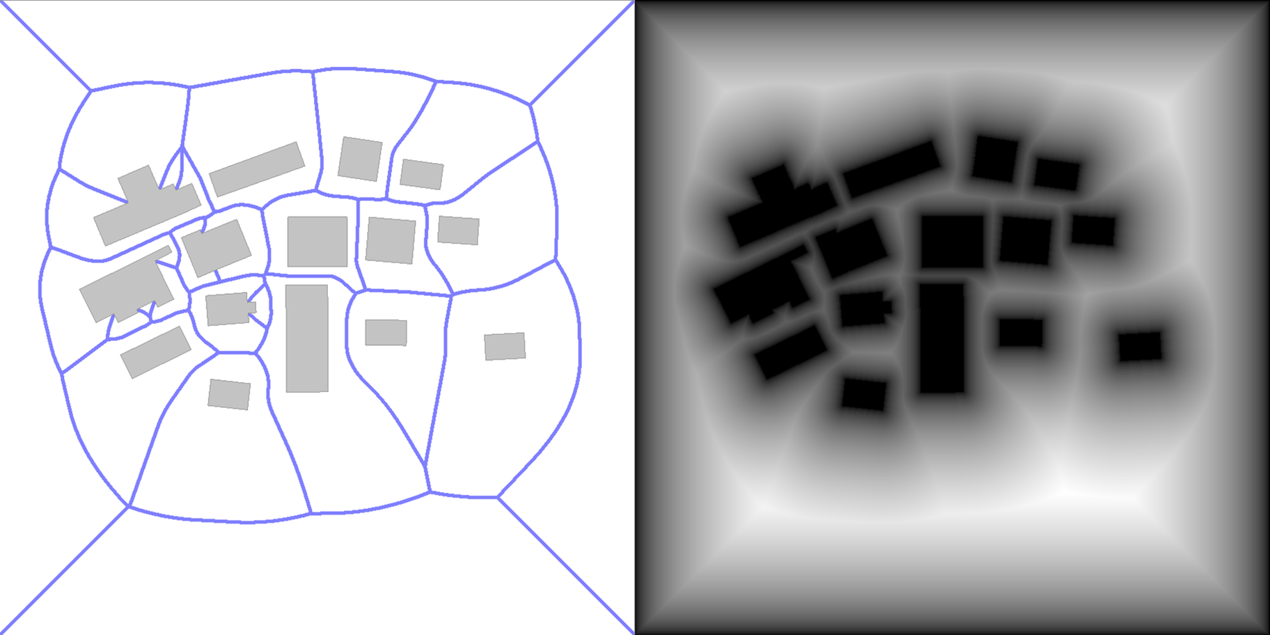
Figure 1: The medial axis (left) and distance map (right) of the same environment
Lucky us, the watershed partitioning method of Recast generates a distance map that we can use. We can use the distance map and partition the scene so that all the region borders fall on an LCM, ensuring all LCMs are covered. One algorithm that allows us to do this is a watershed partitioning algorithm. Recast's built-in watershed formula is optimised for convex regions, resulting in inaccurate segmentations. Thus, I propose a different watershed approach.
Imagine a landscape consisting of hills and valleys. A flood line goes from the lowest to the highest spot, filling each new empty space with water in a region number. All the water gradually grows up while following the flood line. At the top of the hill, two water regions start to touch each other.
Instead of using the height map of the 3D environment, we use the distance map. Using the distance map, we want the local maximum to be the starting point of regions, so we invert the logic. Finally, during the contour trace step (step 5), we check the borders shared between neighbouring areas, which become our LCMs.
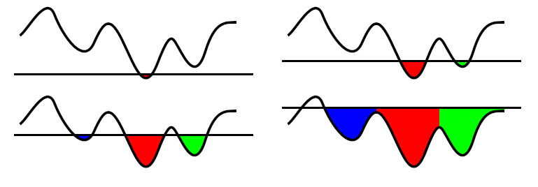
Figure 1: A visualisation of how a watershed works in a 2D environment.
Instead of using the height map of the 3D environment, we use the distance map. Using the distance map, we want the local maximum to be the starting point of regions, so we invert the logic. Finally, during the contour trace step (step 5), we check the borders shared between neighbouring areas, which become our LCMs.
Part 2, Chapter 3: The Tests
We will use environments from other Navmesh studies to evaluate our implementation's accuracy and speed.
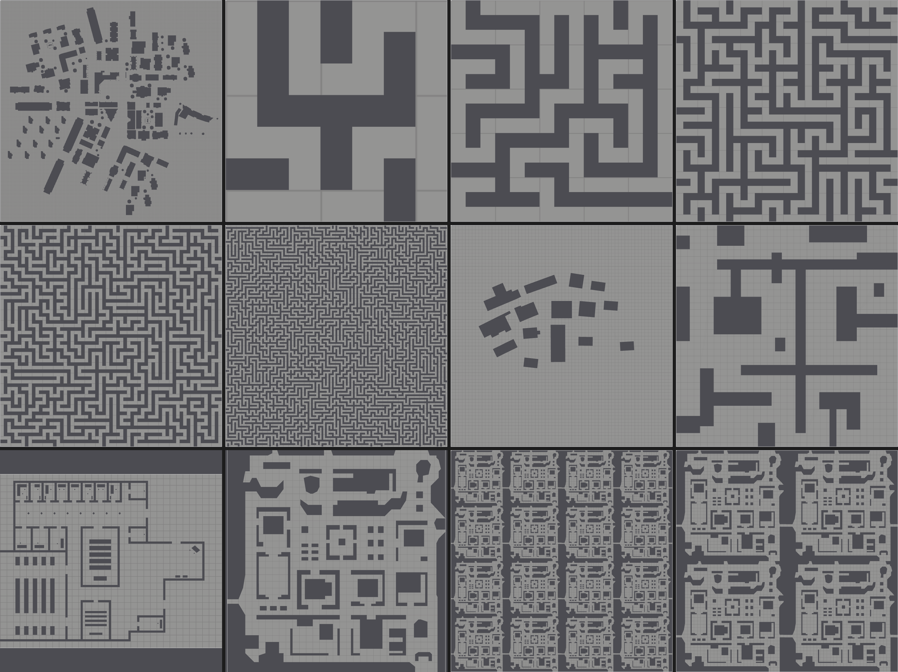
Figure 4: Top view of 2D environments used in the experiments.
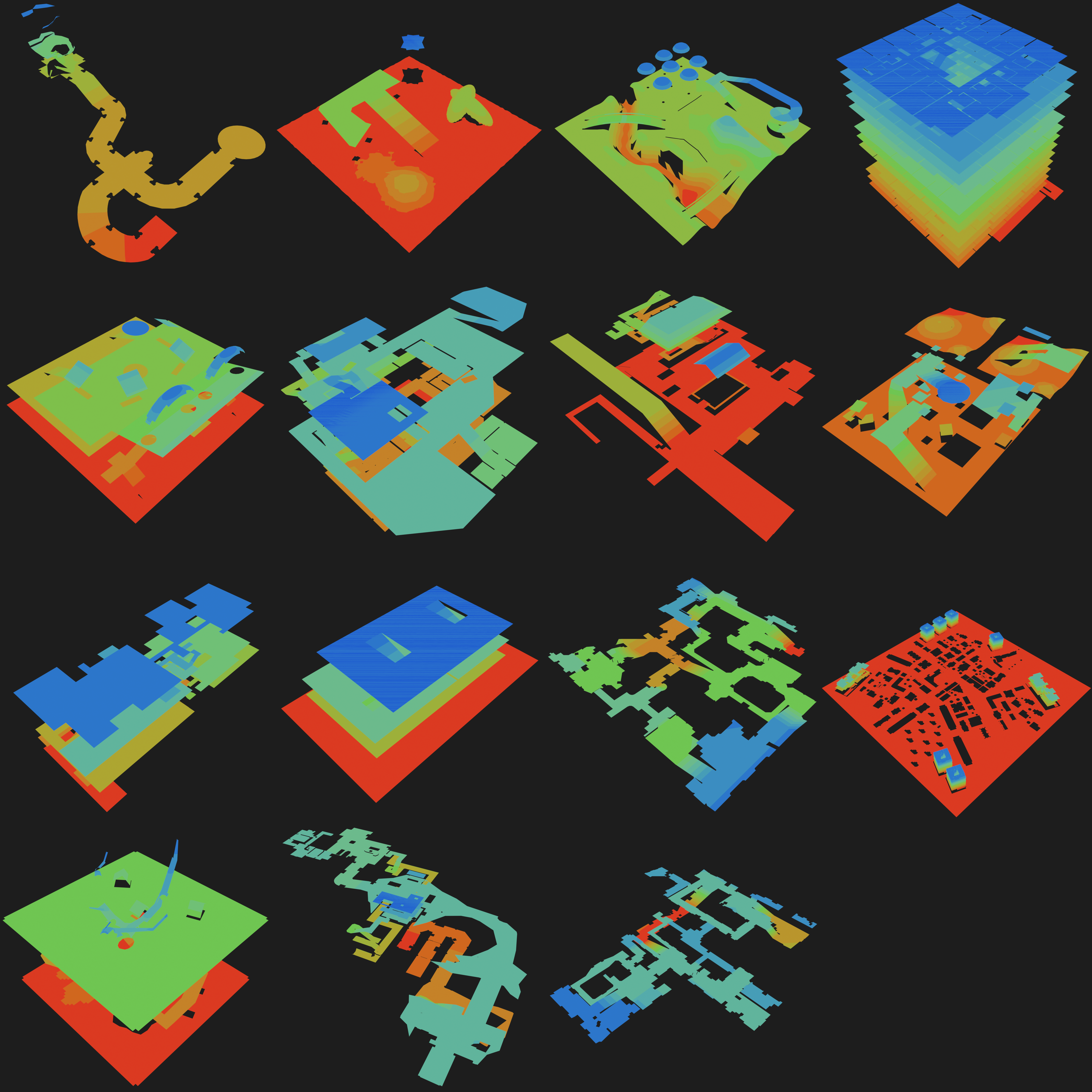
Figure 3: Top view of 3D environments used in the experiments.
The first test measures accuracy by comparing generated LCMs with reference LCMs. The test calculates the distance between the vertices of the generated LCMs and the reference LCMs. If the vertices lie close enough, they are True Positives; if too far, they are False Positives. We can calculate Precision and Recall using the number of True and False positives. The second test runs all environments 100 times, using Recast's built-in timer to measure performance. This test is conducted for our watershed and the built-in watershed to compare performance changes.
Check out the tests on my GitHub fork from Recast for more details on the exact settings.
Part 2, Chapter 4: Results
For full details, read my master's thesis on ResearchGate.
Accuracy:
The results are partly accurate because we only check if the generated LCMs and Reference LCMs are in roughly the same position. Since the comparison does not understand the environment's shape, it can't tell if an LCM is in a saddle segment. A generated LCM in the same saddle segment as the reference LCM might be incorrectly marked as a False Positive if their positions are too far apart. This can happen even though the local clearance is the same. By manually counting the True Positives and False Positives, we can improve the Precision and Recall for all environments. Some environments even achieve perfect scores. We will use auto-generated Precision and Recall values to conclude this experiment.
| Environment | Cell Size | Precision | Recall | Environment | Cell Size | Precision | Recall | Environment | Cell Size | Precision | Recall |
|---|---|---|---|---|---|---|---|---|---|---|---|
| City | 0.1 | - | - | Maze8 | 0.1 | 90.00 | 90.00 | Maze16 | 0.1 | 88.24 | 88.24 |
| 0.2 | 45.23 | 68.39 | 0.2 | - | - | 0.2 | - | - | |||
| 0.3 | 50.88 | 64.14 | 0.3 | 66.67 | 20.00 | 0.3 | 90.00 | 26.47 | |||
| 0.4 | 54.26 | 57.67 | 0.4 | - | - | 0.4 | - | - | |||
| 0.5 | 40.24 | 37.85 | 0.5 | - | - | 0.5 | - | - | |||
| Maze32 | 0.1 | 96.08 | 96.08 | Maze64 | 0.1 | 97.79 | 97.62 | Maze128 | 0.1 | 98.40 | 97.65 |
| 0.2 | - | - | 0.2 | - | - | 0.2 | 64.20 | 10.90 | |||
| 0.3 | 97.50 | 25.49 | 0.3 | 99.32 | 24.79 | 0.3 | 99.81 | 22.17 | |||
| 0.4 | - | - | 0.4 | - | - | 0.4 | - | - | |||
| 0.5 | - | - | 0.5 | - | 0 | 0.5 | - | - | |||
| Military | 0.1 | 15.03 | 76.32 | Simple | 0.1 | 76.67 | 79.31 | University | 0.1 | 85.64 | 71.98 |
| 0.2 | 22.73 | 65.79 | 0.2 | 75.00 | 72.41 | 0.2 | 85.62 | 56.47 | |||
| 0.3 | 24.29 | 44.74 | 0.3 | 75.86 | 75.86 | 0.3 | 82.31 | 46.12 | |||
| 0.4 | 27.27 | 39.47 | 0.4 | 75.00 | 72.41 | 0.4 | 72.73 | 31.03 | |||
| 0.5 | 27.45 | 36.84 | 0.5 | 51.85 | 48.28 | 0.5 | 55.91 | 22.41 | |||
| Zelda | 0.1 | 90.37 | 91.35 | Zelda2x2 | 0.1 | 87.05 | 87.75 | Zelda4x4 | 0.1 | 89.30 | 90.10 |
| 0.2 | 93.79 | 89.73 | 0.2 | 89.32 | 85.75 | 0.2 | 91.20 | 87.41 | |||
| 0.3 | 94.12 | 86.49 | 0.3 | 91.25 | 84.69 | 0.3 | 92.29 | 85.12 | |||
| 0.4 | 89.86 | 71.89 | 0.4 | 86.92 | 70.00 | 0.4 | 89.15 | 71.25 | |||
| 0.5 | 82.50 | 53.51 | 0.5 | 72.78 | 47.07 | 0.5 | 75.53 | 48.72 |
Table 1: Precision and Recall for each environment and cell size.
Our new watershed implementation needs help with misaligned voxel data and input geometry. This results in unassigned grey cells. Over-segmentation in non-axis-aligned areas leads to more False Positives. This lowers Precision due to many local maxima. Smaller cell sizes improve medial axis approximation. However, they increase starting points for new regions. Larger sizes cause heavily aliased edges. This trade-off explains why there is an optimal cell size for Precision. We achieve over 90% Recall in most environments with a Cell Size 0.1.
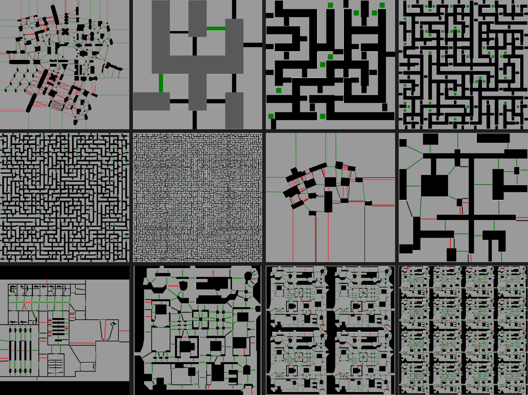
Figure 4: The comparison of LCMs for the 2D environments. Green lines are True Positive, Red lines are False Positive, and Black lines are Reference LCMs without a generated counterpart.
Performance:
Performance data shows variable results: some environments see gains, some losses, and others no change. For instance, City runs faster with the new method, while Big City runs faster with the built-in method. Significance tests reveal that even though you do not notice any difference at large, you can see a difference on a per-sample basis or vice versa. Generally, execution time scales linearly with cell count.

Figure 5: Mean Total, Mean Build Regions, and Mean Build Contours (in milliseconds) between City (left) and Big City (right). The p-value indicates the significance of the independent test. The significance level is 0.05
Part 2, Chapter 5: Conclusions
The current implementation is not recommended for use due to low recall. A low recall can cause agents to clip through environments or enter regions too small. Precision is unpredictable and suffers from over-segmentation. Yet, our performance looks good. While some environments show significant performance changes, the total performance remains similar.
The next chapter (LCM: A Custom Solution from the Ground Up) will explore a new method to generate and extract all LCMs.
Stay tuned!